Cone Calorimeter 101: HRR, THR, and MARHE Explained
What the cone calorimeter measures — heat release rate, total heat release, and MARHE — and why each one matters for fire safety.
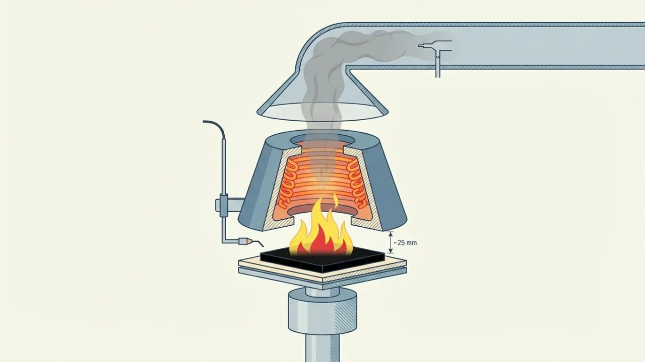
A cone calorimeter turns a 100 mm square of material into a full fire-hazard profile in about fifteen minutes. Three numbers carry most of the story. Peak heat release rate, or pHRR, tells you how fiercely the material burns. Total heat release, or THR, tells you how much fuel it really is. MARHE — the maximum average rate of heat emission — tells you the worst sustained burn across the whole test. Regulators in rail, maritime, and building products all lean on these three numbers. However, none of them means much on its own.
This post walks through each one — what it measures, how labs calculate it, and where it can mislead.
TL;DR
- A cone calorimeter turns a 100 mm sample into a full fire-hazard profile in about 15 minutes.
- Peak heat release rate (pHRR) shows how fiercely a material burns; total heat release (THR) shows how much fuel it really is.
- MARHE — the maximum average rate of heat emission — captures peak, timing, and duration in one number.
- The method rests on oxygen-consumption calorimetry: about 13.1 MJ of heat per kg of O₂ consumed, within roughly ±5%.
- EN 45545-2 anchors European rail fire safety on MARHE, capping it at 90 kW/m² (HL2) or 60 kW/m² (HL3).
- ISO 5660-1, ASTM E1354, and NFPA 271 all describe the same instrument, which Babrauskas built at NBS in 1982.
A bench born at NBS in 1982
The cone calorimeter came out of a simple frustration. Earlier heat-release devices relied on sensible-enthalpy or substitution-burner tricks. They ran, but they drifted by wide margins. As a result, fire labs struggled to compare results across studies.
In 1982, Vytenis Babrauskas at the U.S. National Bureau of Standards (today NIST) tried a different approach. He documented it in NBSIR 82-2611. Instead of closing a thermal energy balance, he measured how much oxygen the specimen’s combustion removed from the exhaust. That switch cut systematic error by an order of magnitude. In 1988, the cone received the R&D 100 Award — the first fire-testing tool ever honoured.
The design soon became an international standard. Today it lives in three parallel documents. First, ISO 5660-1, originally published in 1993 and amended in 2019. Second, ASTM E1354-23 in the United States. Third, NFPA 271 for the fire-protection industry. All three describe the same instrument.
The name comes from its radiant heater — a truncated conical electrical element wound so the smaller aperture points down at the specimen, 25 mm below. The cone shape delivers a nearly uniform radiant flux (±2%) on a flat 100 × 100 mm sample. Moreover, labs can program the flux anywhere from 0 to 100 kW/m². Standard test fluxes sit at 25, 35, 50, and 75 kW/m². These match, in order, an early fire, a developing compartment fire, the onset of flashover, and a severe post-flashover exposure. A 10 kV spark igniter hangs above the specimen, and the lab conditions the whole sample for at least 48 hours at 23 °C and 50% relative humidity before each test.
Why oxygen tells the heat story
The trick that makes the cone work is older than the cone itself. Back in 1917, the British chemist W. M. Thornton noticed something strange. Most organic fuels, no matter how different they looked, released about the same amount of heat per kilogram of oxygen consumed. In 1980, Clayton Huggett extended that rule to solids. He nailed the number down to 13.1 MJ per kilogram of oxygen, with a standard deviation of only 0.35 MJ/kg — about ±5%.
That constancy is the whole game. Ignition chemistry, soot yield, and char fraction vary wildly from fuel to fuel. However, the per-oxygen energy release does not. Therefore, you can skip the thermal balance entirely. Instead, you simply track how much oxygen disappears from the exhaust duct, then multiply by 13.1.
W. J. Parker put the math on paper in 1984. His formula still runs inside every cone calorimeter’s software today.
In plain terms: is the 13.1 MJ/kg-O₂ constant, is the oxygen depletion factor (how much oxygen the flame has stripped from the incoming air), is the expansion factor that accounts for combustion’s volume change, is the incoming air mass flow, and is the ambient oxygen mole fraction. In 1991, Marc Janssens added a correction for incomplete combustion. When the exhaust contains carbon monoxide, his formula adds a second constant, MJ/kg-O₂ — the extra heat that CO would have given off if it had burned all the way to CO₂. In 2016, the DiNenno Prize recognised oxygen-consumption calorimetry as one of fire science’s most consequential ideas.
Hardware that implements the physics
A modern cone calorimeter runs as a quiet symphony of sensors. A paramagnetic analyser tracks oxygen in the exhaust with excellent linearity. Two NDIR sensors watch carbon monoxide and carbon dioxide. A strain-gauge load cell, resolved to 0.1 g, logs the specimen’s mass loss in real time. An orifice plate with a differential-pressure transducer feeds the exhaust mass flow into the formula above. Finally, a 632.8 nm helium–neon laser photometer in the duct measures smoke obscuration. That photometer — which Babrauskas and Mulholland added in 1987 — explains why the current ISO 5660-1 title now explicitly includes “smoke production rate (dynamic measurement)”.
Heat release rate: the most important number
If a cone calorimeter had to report only one number, that number would be heat release rate, or HRR. In a widely cited 1992 paper, Babrauskas and Peacock called HRR “the single most important variable in characterizing the flammability of products and their consequent fire hazard.” At first, that claim sounds wrong. After all, most fire deaths come from smoke and toxic gases, not from flames.
However, HRR is the best predictor of how fast a fire grows toward those lethal conditions. Once a room fire really takes off, smoke and carbon monoxide arrive in large quantities regardless of a material’s specific toxic potential. Therefore, the metric that tracks growth rate wins. Peak HRR, or pHRR, is simply the maximum of the HRR curve over the test. It governs whether a room will reach flashover, and it drives the radiative feedback that ignites nearby fuels. Time-to-flashover in the ISO 9705 room-corner test, for instance, correlates strongly with cone pHRR.
Reading the HRR curve shape
A raw HRR curve tells more than its peak. Schartel and Hull laid out a four-part taxonomy in 2007 that fire labs still use.
Thermally thin materials — textiles, thin films, collapsed foams — produce a single sharp peak. The whole specimen pyrolyses almost at once. As a result, available fuel sets pHRR rather than the steady burning physics.
Thick non-charring polymers — thick cast PMMA is the classic example — burn in a broad plateau. Once the pyrolysis zone reaches thermal balance with the imposed flux, burning settles into a quasi-steady state.
Thick charring solids — wood and many composites — show a characteristic two-peak shape. First, surface pyrolysis produces a peak as the outer layer degrades. Then an insulating char forms, the HRR dips, and the pyrolysis front drives deeper. Finally, when the thermal wave reaches the back face, a second peak — often higher than the first — emerges as the backing radiates the heat forward.
Intumescent systems flip the script. They show a small early peak before the expanding char swells up and blocks both heat and volatiles. The result is dramatic suppression. For example, recent biomass-based intumescent coatings cut pHRR by 83–90% compared with the uncoated substrate.
Typical pHRR values at 50 kW/m² span nearly two orders of magnitude. Neat polypropylene burns fiercely at about 1,275 kW/m², and polyethylene lands between 900 and 1,400. Cast PMMA settles into its quasi-steady range of 650–900 kW/m². Rigid polyurethane foam runs 370–740 kW/m², while solid pine peaks modestly at 150–250. On the other end, glass-fibre/phenolic aircraft composites stay under 200 kW/m², but a carbon-fibre/iPP composite hit 1,738 kW/m² in a 2019 study.
The danger of quoting cone calorimeter pHRR alone: it rewards transient spikes. A 1.6 mm HIPS specimen can hit 1,200 kW/m² and burn out in 90 seconds. Meanwhile, a 25 mm charring insulation board may never exceed 150 kW/m² and still release five times more total energy. In short, the peak is only half the story. To see the rest, we need to add up the whole curve.
Total heat release: the fuel load in one integral
Peak heat release rate captures how fiercely a material burns. However, it says nothing about how long. That is where total heat release, or THR, comes in. THR is simply the time integral of HRR, expressed in megajoules per square metre of exposed specimen.
In plain terms, THR is the area under the HRR curve. It represents the total fire load that the specimen contributes per unit exposed area — the energy available if the material burns to completion under the test’s ventilation. That makes THR directly useful to fire engineers. For example, the parametric fire curves in Eurocode EN 1991-1-2 build their design fire-load densities from data of exactly this kind.
THR also links to a deeper property called the effective heat of combustion, or EHC. In plain terms, EHC divides total heat output by total mass burned off during the test.
Here is the specimen’s exposed area and is the mass it lost. EHC is always lower than the gross heat of combustion from a bomb calorimeter. The ratio between them is the combustion efficiency , typically 0.7–0.95 for well-ventilated flaming.
The diagnostic power of EHC is what makes flame-retardant (FR) science tractable. A drop in EHC with added flame retardant signals gas-phase action — halogens or phosphorus compounds disrupting radical chemistry inside the flame. In contrast, a THR reduction without an EHC change points to condensed-phase action: char formation, or heat-sink fillers like aluminium hydroxide (ATH) and magnesium hydroxide (MDH). Schartel and Hull and FAA report AR-05/14 lean on this exact split when they certify new FR systems.
THR also complements pHRR where pHRR misleads. A low-pHRR, high-THR material burns slowly for a long time and still delivers a large total fuel load. Conversely, a high-pHRR, low-THR material flashes and dies. Therefore, regulators often report THR inside fixed time windows. EN 13823 SBI uses THR at 600 seconds (THR₆₀₀ₛ). Meanwhile, IMO FTP Code Part 5 imposes Q_t ≤ 0.7 MJ for bulkhead linings and ≤ 2.0 MJ for deck and floor coverings. Same idea, different windows.
MARHE: the metric that captures intensity and duration
Two numbers still fall short. pHRR is too spiky, and a simple average HRR gets diluted by long low-emission tails. Neither reliably predicts how a material will behave at full scale. Fire scientists needed a single scalar that combined peak, timing, and duration into one fair number. That scalar is MARHE — the maximum average rate of heat emission.
The math is two steps. First, define the average rate of heat emission from test start:
Then take its maximum over the whole test:
In plain terms, ARHE is a running average of the HRR curve from the beginning of the test. MARHE captures the highest value that running average ever reaches. Because ARHE accumulates heat before it maximises, a single number ends up sensitive to four things at once: time-to-ignition, peak intensity, total heat released, and when the peak happens. An early sharp peak raises MARHE much more than a late one does.
That is precisely what correlates with full-scale fire behaviour. As Luo and colleagues put it in 2022, MARHE “objectively and comprehensively reflects the heat release performance of the samples in the whole combustion process.” A Nordtest screening study found MARHE to be the second most important cone predictor of SBI and room-corner-test performance, behind only pHRR.
Why EN 45545-2 chose MARHE
That correlation with full-scale fire outcomes is why MARHE anchors EN 45545-2, the European railway fire-safety standard. Measured per ISO 5660-1 at 50 kW/m², MARHE serves as the principal pass/fail heat-release parameter for most of the 26 requirement sets (R1–R26). Each set also gets graded by hazard level — HL1 for low risk, HL2 for standard passenger trains, HL3 for long-tunnel or underground services.
The thresholds run tight. The table below shows a representative slice.
| Requirement set | Application | HL2 | HL3 |
|---|---|---|---|
| R1 (interior vertical/horizontal surfaces) | Side walls, partitions, interior doors | MARHE < 90 kW/m² | MARHE < 60 kW/m² |
| R6 (seat shells F1C/F1D) | Passenger seat shell base and back | MARHE < 90 kW/m² | MARHE < 60 kW/m² |
| R7 (exterior surfaces, gangway interiors) | Body-shell walls, gangways | MARHE < 90 kW/m² | MARHE < 60 kW/m² |
The U.S. FRA report DOT/FRA/ORD-19/39 reproduces the full set. For complete seats, EN 16989 also reports MARHE in kilowatts alongside total smoke production. In maritime practice, MARHE appears in Part 10 of the IMO 2010 FTP Code for fire-restricting materials on high-speed craft. Part 5 of the same code, however, sticks to a different radiant-panel method with Q_p and Q_t. Different scenarios, different metrics — but MARHE keeps winning the battles where time and temperature both matter.
The other parameters worth knowing
A full cone calorimeter report reads more like a material fingerprint than a single number. Several supporting cone calorimeter metrics travel with HRR, THR, and MARHE.
Time to ignition (TTI), in seconds, scales with thermal inertia and the square of the ignition-temperature difference. Below a critical heat flux of roughly 10–20 kW/m², most polymers and cellulosics will not ignite at all.
Mass loss rate, in g/m²·s, paired with EHC, diagnoses FR mechanism — the same gas-phase vs condensed-phase split we saw earlier.
Smoke production rate (SPR), its integral TSP, and specific extinction area (SEA) describe visibility loss. SEA hovers around 100 m²/kg for clean-burning PMMA. Meanwhile, it soars past 1,000 m²/kg for aromatic polymers like PVC and polystyrene. Those same materials also dump more soot and CO into the smoke layer.
CO and CO₂ yields, in kg per kg of burned mass, quantify how completely the fuel burns. Under vitiated atmospheres — the topic of ISO/TS 5660-5:2020, the controlled-atmosphere cone — CO yields from PMMA more than double as the oxygen concentration drops from 21% to 14%. In other words, an underventilated compartment does not just burn slower; it also produces much more toxic CO.
Finally, the Fire Growth Rate Index (FIGRA) deserves a mention. Formally, EN 13823 SBI defines FIGRA as the maximum of HRR(t) divided by t. Labs routinely compute a cone calorimeter version as pHRR over time-to-peak or time-to-ignition. In their 2007 NIST study of UL-94-rated plastics, Morgan and Bundy recorded cone calorimeter FIGRA values spanning from about 0.5 kW/(m²·s) for a bromine-FR V-0 polycarbonate to 16 kW/(m²·s) for non-FR polypropylene. That thirty-fold spread shows how dramatically fire growth rate varies even between materials with similar pHRR.
Typical cone calorimeter values at 50 kW/m²
For a sense of scale, here is where common materials land. All numbers come from cone calorimeter tests at 50 kW/m² in horizontal orientation.
Plastics and foams:
| Material | Thickness | TTI (s) | pHRR (kW/m²) | THR (MJ/m²) | EHC (MJ/kg) |
|---|---|---|---|---|---|
| PMMA (cast, black) | 25 mm | 50–90 | 650–900 (quasi-steady) | 800–1,200 | ~24 |
| HDPE | 5 mm | 60–80 | 900–1,400 | 130–160 | ~40 |
| Polypropylene (neat) | 3.2 mm | 25–50 | 1,275–2,200 | 120–150 | ~40–46 |
| PVC (non-FR) | 3.2 mm | 23 | 243 | 51 | 14 |
| Rigid PUR foam | 25 mm | 2–5 | 370–740 | 30–80 | 15–20 |
| Flexible PUR foam | 20 mm | 2–10 | 200–450 | 20–40 | 20–25 |
Wood products and composites:
| Material | Thickness | TTI (s) | pHRR (kW/m²) | THR (MJ/m²) | EHC (MJ/kg) |
|---|---|---|---|---|---|
| Pine / spruce (solid) | 10–18 mm | 20–40 | 150–250 (two peaks) | 40–100 | 12–15 |
| OSB / plywood (untreated) | 11–18 mm | 30–60 | 170–250 initial peak | 50–90 | 12–15 |
| FRT wood composite | 11–18 mm | >50 | 300-s avg 58–100 | 30–40% reduced | reduced |
| GFRP / phenolic (aircraft) | 2–4 mm | 50–100 | 100–200 | 10–25 | 8–15 |
Treat these cone calorimeter numbers as representative ranges, not rigid material constants. Grade, thickness, pigment, and backing all shift them.
In practice, combined standard uncertainty on pHRR sits at 5–10% inside a single laboratory. Inter-laboratory round-robins push that spread out to 15–25% for TTI and THR. For this reason, a good cone report always gives the mean of three replicates along with the heat flux, specimen thickness, retainer-frame status, and backing material. Without that context, two numbers from two labs cannot fairly share a page.
Pitfalls that skew cone calorimeter results
No measurement is innocent. Edge effects and specimen preparation drive most of the error in cone calorimeter results. The retainer frame covers only a few millimetres of specimen edge, and for composites and sandwich panels, pyrolysis gas escaping from the sides can add spurious early HRR. Both Tsantaridis and Sandinge and colleagues in 2022 quantified swings of 10–15% between framed and unframed tests. For this reason, every report must state the frame configuration.
Moisture content governs TTI. Conditioning to 23 °C and 50% relative humidity for 48 hours stays non-negotiable. Substrate choice also matters. Standard ceramic fibre backing versus an aluminium plate visibly reshapes the second peak of charring thick specimens.
Intumescent coatings expand toward or beyond the 25 mm cone-to-specimen gap, effectively raising the flux on the specimen surface. Some labs handle this by using a 50 mm gap or inserting a wire grid above the sample. Meanwhile, thermoplastics that melt and drip require the 5 mm aluminium foil edge lip to keep molten polymer from flowing out of the holder.
Sample thickness matters profoundly. In the Schartel and Hull taxonomy, PMMA at 1.5 mm produces a fuel-limited sharp peak. At 6 mm, the same material shows a broader single peak. At 25 mm, it settles into the near-steady plateau discussed earlier. Same polymer, three completely different HRR curves. This is why reporting specimen thickness alongside every number matters.
From 100 cm² to a real fire
A 100 mm square is not a building. The cone calorimeter is a bench-scale, well-ventilated, one-dimensional forced-flaming test. It does not reproduce wall re-radiation, enclosure feedback, oxygen vitiation, or multi-dimensional flame spread. Flame heat-flux feedback on the cone specimen runs only about 19–37 kW/m², depending on polymer. In contrast, flashover rooms routinely see 40–100 kW/m². That gap shapes how fire engineers use cone data.
Intermediate-scale bridges help close the gap. The EN 13823 SBI test burns a 1.5 m corner specimen with a 30 kW propane sandbox. It produces the FIGRA, THR₆₀₀ₛ, and SMOGRA numbers that drive the Euroclass A2/B/C/D classification of building products. Moreover, Efectis offers correlation software that predicts SBI behaviour from a single cone HRR history. Twelve 0.01 m² cone specimens can replace three 2.25 m² SBI specimens.
At full scale, the ISO 9705 room-corner test remains the reference. And this is precisely why MARHE exists — to make small cone calorimeter data useful for these larger-scale fire predictions in the first place.
Key takeaways
A competent cone calorimeter report never reduces a material to one number. First, pHRR tells you how fiercely the material peaks. Second, THR tells you how much total fuel it really is. Third, MARHE tells you the worst sustained burn rate across the whole test. Next, TTI tells you how quickly the material gets there. Then, EHC tells you whether a flame retardant works in the gas phase or the condensed phase. Finally, SEA, CO yield, and CO₂ yield describe the smoke and toxic hazard. In short, each number has a job.
Regulators choose their metric to match the scenario. EN 45545-2 anchors on MARHE because rail fires burn for minutes in confined tunnels. IMO FTP Part 5 limits Q_t and Q_p because ship linings must not push a compartment toward flashover. Euroclass rests on SBI-derived FIGRA and THR₆₀₀ₛ because building products matter most in the first ten minutes of fire growth. Understanding why each metric exists — and reading the shape of the HRR curve rather than just its peak — is what separates a fire safety engineer from a data consumer. More than forty years after Babrauskas built the first cone, that is still the instrument’s enduring value.
Cite this article
Dinh, D. C. (2026, April 18). Cone Calorimeter 101: HRR, THR, and MARHE Explained. PyroRisk. https://pyrorisk.net/blog/cone-calorimeter-101/
Recent posts
Featured posts
Categories
Comments
Related posts
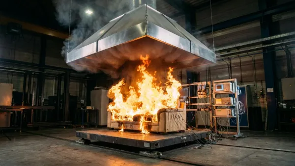
Heat Release Rate: Why HRR Is the King of Fire Science
Why heat release rate is the single most important number in fire science: how labs measure it, what it predicts, and why it outranks smoke toxicity.
The Science of Fire: What You Think You Know Is Wrong
Explore the science of fire — from radical chain reactions and flame anatomy to flashover physics and why modern homes burn 7x faster than 1950s ones.
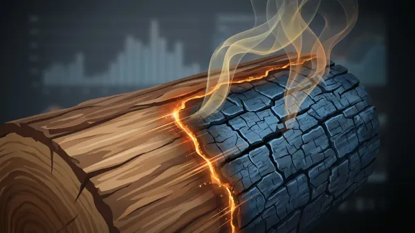
The Science of Pyrolysis: How Heat Unmakes Everything
Pyrolysis — heat breaking molecular bonds without oxygen — drives wildfires, battery thermal runaway, biochar, plastic recycling, and even coffee roasting.