F-N Curve and Societal Risk: Drawing the Line on Safety

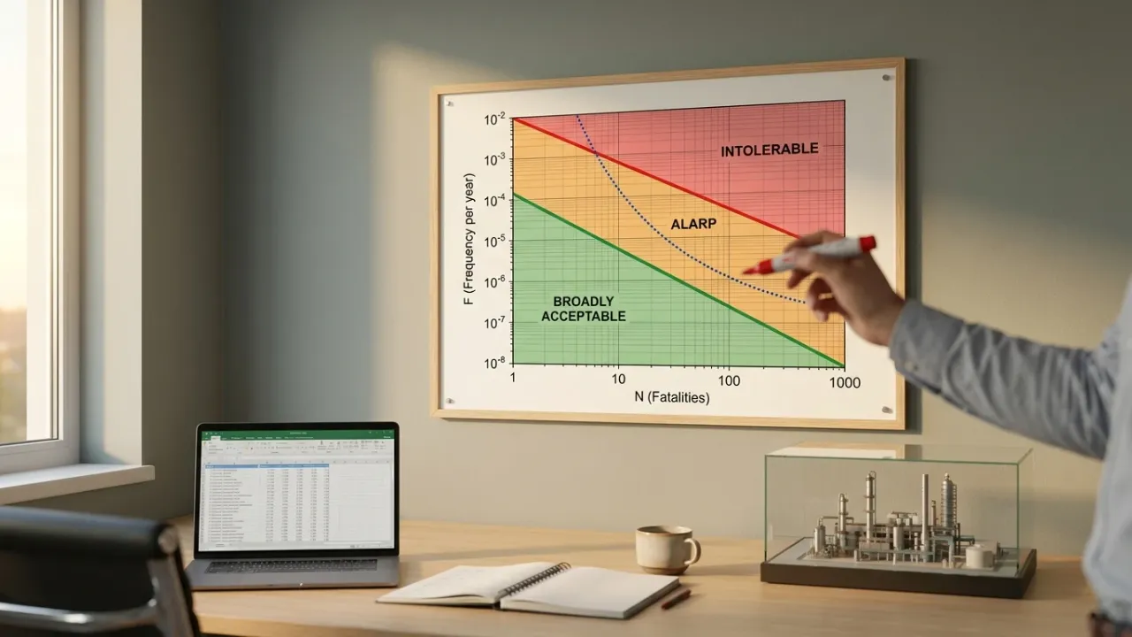
How safe is safe enough? Every engineer who works on a major hazard meets that question sooner or later. Physics alone cannot answer it. You can always add redundancy, distance, or extra checks. So the real question asks whether the next slice of safety earns its cost. It also asks whether today’s societal risk falls inside what the public will accept. An F-N curve turns that judgement into a chart. ALARP then turns the chart into a rule. This post walks through the math, the slope, and the anchor numbers that offshore, nuclear, and rail actually use.

TL;DR

• An F-N curve plots the yearly frequency F of accidents killing N or more people, on log-log axes.
• The slope α encodes risk aversion. At α = 1, a tenfold bigger disaster must occur tenfold less often; at α = 2, a hundredfold.
• The ALARP carpet sits between an intolerable line and a broadly acceptable line, two to three decades apart.
• UK HSE calls 1 in 1,000,000 per year broadly acceptable for one person.
• Dutch law enforces F(N)·N² ≤ 10⁻³ per year at roughly 4,000 sites.
• The worked plant below clears the UK line, but breaks the Dutch line three times.
• Piper Alpha killed 167 of 226 people in 1988 and rewrote North Sea law.
• US NRC caps core damage frequency at 10⁻⁴ per year, large early release at 10⁻⁵.
• EU rail sets no common numbers. CSM-RA harmonises the process instead.

What does an F-N curve plot?

An F-N curve plots the yearly frequency F of accidents that kill N or more people. Both axes run on a log scale. So the curve shows the full shape of societal risk, not just its average. Write f(n) for the annual chance of an accident that kills exactly n people. The curve then reads:

$F(N) = P(\text{fatalities} \ge N) = \sum_{n=N}^{\infty} f(n) \quad \text{per year}$

So F(N) gives the complementary cumulative distribution of yearly deaths. Most engineers shorten that to CCDF. For a smooth consequence model, the sum simply becomes an integral.

The “or more” rule does two jobs. First, it removes binning artefacts, since nobody has to decide whether 47 deaths belong in the 40s bucket or the 50s. Second, it forces the curve to fall from left to right. Both properties therefore make curves from different studies comparable. The shape first reached a wide public in the 1975 WASH-1400 reactor study, and it has anchored societal risk work ever since.

How do you build one from a QRA?

You build an F-N curve straight out of an event tree, one branch at a time. Each branch gives a frequency and a fatality count. Then you sort and add.

Take a small process plant with four modelled outcomes. The frequency column comes from fault tree and event tree work. Meanwhile the fatality column comes from consequence modelling — fire, blast, and smoke exposure.

Scenario	Frequency (per year)	Fatalities N
Small leak, local pool fire	3 × 10⁻⁴	1
Jet fire on the process deck	4 × 10⁻⁵	8
Vapour cloud explosion	6 × 10⁻⁶	25
Riser rupture, total loss	5 × 10⁻⁷	60

Now add from the bottom up, because every scenario with 8 or more deaths counts toward F(8). That gives four points:

• F(1) = 3.47 × 10⁻⁴ per year
• F(8) = 4.65 × 10⁻⁵ per year
• F(25) = 6.5 × 10⁻⁶ per year
• F(60) = 5 × 10⁻⁷ per year

Plot those four points on log-log paper and you hold the plant’s societal risk curve. Real studies run hundreds of branches, so the result looks smooth. Still, the method never changes.

Why do PLL and FAR compress societal risk?

PLL and FAR each squeeze the whole F-N curve into one number. That makes them easy to compare, but also easy to misread. Integrate the curve and you get expected deaths per year. Safety engineers call that the Potential Loss of Life, or PLL:

$\text{PLL} = E[N] = \sum_{n=1}^{\infty} n \cdot f(n) = \int_{0}^{\infty} F(N)\, dN$

For the four-branch plant above, the sum runs 3 × 10⁻⁴ + 3.2 × 10⁻⁴ + 1.5 × 10⁻⁴ + 3 × 10⁻⁵. So PLL lands at 8.0 × 10⁻⁴ deaths per year. Note what the number hides, though. Three of the four branches contribute more than the big one, yet the rare 60-fatality case drives every public argument about the site.

PLL gives the area under the F-N curve on linear axes. But it cannot tell one 1,000-death disaster from a thousand single-death accidents. So the offshore world prefers the Fatal Accident Rate, or FAR, which rescales PLL per 10⁸ exposure hours. That figure stands for roughly a thousand working lifetimes. For example, IOGP reported a 2019 upstream FAR of 0.82, down from 1.01 the year before. Both measures serve cost-benefit work well. Yet neither one flags catastrophe potential, so regulators keep the curve as well as the scalar.

What does the slope α mean?

The slope α sets how harshly a criterion punishes large accidents. Most regulatory limits therefore run as straight lines on log-log paper:

$F(N) \le \frac{C}{N^{\alpha}}$

Here C fixes the height of the line and α fixes its tilt. Take logs and the geometry falls out. Two values then dominate practice:

$\log F = \log C - \alpha \log N$

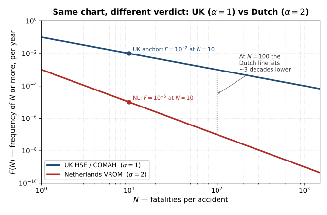
• α = 1, risk-neutral. A tenfold larger accident must occur tenfold less often. So the line holds expected deaths flat, and it treats one 10-death event and ten 1-death events alike.
• α = 2, risk-averse. A tenfold larger accident must occur a hundredfold less often. Society then penalises catastrophes far harder than expected value alone would.

Dutch policy runs on α = 2, as Bottelberghs (2000) sets out. UK HSE, in contrast, runs its COMAH guidance on α = 1. Parts of the UK ACDS port framework split the difference, with α = 1 for small N and α = 2 above a breakpoint. Whether α > 1 can be defended at all has fuelled a thirty-year argument. A slope steeper than −1 says, quite literally, that one crash killing 10 people counts as worse than ten crashes killing one each.

There also sits a neat piece of theory under the straight lines. When accident severity follows a power law — a Pareto jump distribution on a compound Poisson process — the F-N curve comes out straight on log-log axes by construction. Braband and Schäbe used exactly that result to derive railway criteria from European accident data.

Same plant, two verdicts

Slope choice decides real cases, not just arguments. So score the four-branch plant against both lines, and the point lands hard. The UK COMAH line runs at slope 1 through F = 10⁻² per year at N = 10, so its limit reads 10⁻¹/N. The Dutch line, meanwhile, reads 10⁻³/N².

N	Plant F (per year)	UK limit, α = 1	Dutch limit, α = 2	Verdict
1	3.47 × 10⁻⁴	1 × 10⁻¹	1 × 10⁻³	Passes both
8	4.65 × 10⁻⁵	1.25 × 10⁻²	1.6 × 10⁻⁵	Fails Dutch, 3× over
25	6.5 × 10⁻⁶	4.0 × 10⁻³	1.6 × 10⁻⁶	Fails Dutch, 4× over
60	5.0 × 10⁻⁷	1.7 × 10⁻³	2.8 × 10⁻⁷	Fails Dutch, 1.8× over

One curve. Two regulators. Two answers. The plant clears the UK line by two to three decades at every point, yet breaks the Dutch line almost everywhere above a single fatality. Nothing about the physics changed. Only α did.

What is the ALARP carpet?

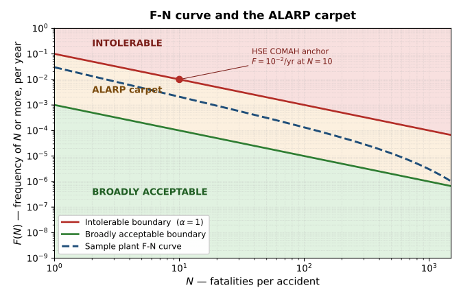
The ALARP carpet names the band between an intolerable line and a broadly acceptable line on the same F-N chart. Risks inside it pass only after real reduction effort. So plot two parallel lines with the same slope −α:

$F_{\text{int}}(N) = \frac{C_{\text{int}}}{N^{\alpha}}, \qquad F_{\text{ba}}(N) = \frac{C_{\text{ba}}}{N^{\alpha}}$

Regulators usually set C_int two to three orders of magnitude above C_ba. The strip between them forms the carpet. Above it, no benefit buys authorisation. Below it, further spending buys little. Inside it, though, the operator must cut risk as low as reasonably practicable. The same idea appears as the familiar triangle in HSE’s Reducing Risks, Protecting People (R2P2), and HSE’s individual-risk anchors now read like textbook furniture:

• 1 in 1,000 per year — intolerable for a worker.
• 1 in 10,000 per year — intolerable for a member of the public.
• 1 in 1,000,000 per year — broadly acceptable for anyone.

For societal risk, R2P2 offers a single guidance point. An accident killing 50 or more people, at a frequency above 1 in 5,000 per year, lands in the intolerable zone. From that anchor, HSE’s 2012 COMAH guidance extends a slope-1 line through F = 10⁻² per year at N = 10, and then puts the broadly acceptable line two decades lower.

How does gross disproportion work?

Gross disproportion means the duty-holder must spend past the plain cost-benefit break-even point. The multiplier then grows with the risk.

Inside the carpet, a bare cost-benefit test would reject any measure whose cost exceeds its monetised benefit. UK practice rejects that logic. A measure counts as reasonably practicable unless its cost sits grossly disproportionate to the risk it removes. So duty-holders near the intolerable line apply a larger factor than those near the broadly acceptable line. In short, the closer you sit to the top of the carpet, the more you must spend to stay there.

Where did the F-N curve come from?

Four milestones bracket the modern framework, and each one followed a real dispute rather than a theory.

1967 — Farmer’s siting paper. F. R. Farmer, at the UK Atomic Energy Authority, asked how iodine-131 release size should trade against release frequency when siting reactors. His answer, given at the IAEA Vienna symposium in April 1967, drew a near-inverse line: twice the consequence, at most half the frequency. People still call the chart a Farmer diagram.

1975–77 — WASH-1400 and Kendall. The Rasmussen study redrew Farmer’s idea on log-log axes, then set reactor risk beside dam failures, fires, and air crashes. Kendall and colleagues turned the same construction on regulation more broadly. So for the first time, an F-N chart carried a public argument about tolerability across different hazards.

1978–81 — the Canvey Island studies. HSE commissioned the first full probabilistic assessment of a non-nuclear industrial complex in 1976. The Canvey reports delivered individual-risk contours and societal risk curves for a refinery and methane terminal on the Thames Estuary. The second report, in 1981, revised the method and lowered the assessed risk. Every major-hazard QRA since has copied that template.

1992–2001 — TOR, the Royal Society, and R2P2. HSE’s Tolerability of Risk from Nuclear Power Stations answered Sir Frank Layfield’s recommendation from the Sizewell B inquiry. Meanwhile the Royal Society study group consolidated the academic view. Then in 2001, R2P2 generalised the framework to every work activity in Britain.

The Netherlands took a different road and wrote the framework into law. VROM fixed a hard individual location-risk limit of 10⁻⁶ per year, plus the societal risk guideline F < 10⁻³/N². Those rules now cover roughly 4,000 hazardous establishments, and since 2006 RIVM has mandated the SAFETI-NL software to apply them. Jonkman, Jongejan and Maaskant later carried the same criterion into flood-defence policy. So one line now bounds dyke, plant, and tunnel risk within a single frame.

How does offshore draw the line?

Offshore practice grew out of one night. On 6 July 1988, gas leaked from a condensate pump on the Piper Alpha platform and ignited. The blasts killed 167 of the 226 people aboard.

That wreck changed the law. Regulation of UK offshore safety moved from the Department of Energy to HSE in 1991. The Offshore Installations (Safety Case) Regulations followed in 1992. Lord Cullen’s inquiry produced 106 recommendations, and the government accepted all 106. Cullen also pushed regulators away from prescriptive checklists, toward goal-setting risk work. As a result, operators spent an estimated £1 billion in the immediate aftermath.

Today every UK duty-holder must file a quantitative risk assessment that shows three things. First, individual risk per annum for the most exposed worker sits inside the ALARP region, below the 10⁻³ per year intolerable line. Second, societal risk curves for major-accident hazards stay clear of HSE’s uncomfortably high zone. Third, cost-benefit analysis with a gross-disproportion factor supports the ALARP claim. The regime famously specifies the question, yet leaves the answer open.

Norway runs a parallel system. Its regulator, the Petroleum Safety Authority, became Havindustritilsynet — Havtil — on 1 January 2024. The numerical machinery comes from NORSOK Z-013, the standard for risk and emergency preparedness assessment on the Norwegian shelf. Z-013 deliberately leaves the numbers to the operator. Still, industry practice has converged anyway:

• IRPA near 1 × 10⁻³ per year as a limit for the most exposed group, with an ALARP objective near 1 × 10⁻⁵ per year.
• Group FAR for a platform below 10 per 10⁸ exposure hours.
• Third-party societal risk plotted against a slope-1 line through F = 10⁻⁴ per year at N = 10, with the broadly acceptable line two decades lower.

The Z-013 vocabulary — IRPA, FAR, PLL, MSF for main safety function, DAL for dimensioning accidental load — has become standard North Sea shorthand. Trbojevic’s comparison of EU criteria found the same pattern in both regimes. Individual risk works as a hard limit, while societal risk works as a curve, and ALARP does the rest.

How does nuclear draw the line?

Nuclear regulators wrap the same geometry in different vocabulary, and they mostly work through surrogate targets rather than the F-N curve itself.

The IAEA sets the frame. Its Fundamental Safety Principles (SF-1, 2006) list ten principles, including limitation of individual risk and optimisation of protection. SSR-2/1, revised in 2016, turns those into design requirements. Its post-Fukushima text pushes hard on “practical elimination” of conditions that could cause an early or large release.

The US NRC adopted numerical Safety Goals in 1986, backed by two Quantitative Health Objectives:

• Prompt fatality QHO. Risk to an average person within about 1 mile must stay under 0.1% of all-cause accidental death risk. Against a 1980s baseline near 5 × 10⁻⁴ per year, that implies about 5 × 10⁻⁷ per reactor-year.
• Latent cancer QHO. Cancer risk to the population within about 10 miles must stay under 0.1% of background cancer risk, or roughly 2 × 10⁻⁶ per reactor-year.

Checking those directly needs a Level 3 PRA, which costs a great deal. So the NRC defines two plant-level surrogates instead. Core damage frequency must stay below 10⁻⁴ per year. Large early release frequency must stay below 10⁻⁵ per year. In practice the US fleet beats both by about a decade, with CDF near 10⁻⁵ and LERF near 10⁻⁶. For new builds, the NRC and IAEA both expect design CDF under 10⁻⁵ per year.

The UK ONR reaches the same place with its own words. Its Safety Assessment Principles define Basic Safety Levels as the boundary above which risk turns intolerable, and Basic Safety Objectives as the level below which further cuts normally stop. Numerical Targets 4 to 9 cover individual and societal risk for workers and the public alike. That lineage runs straight back to the 1992 Tolerability of Risk document, benchmarked against IAEA standards and WENRA reference levels.

Dutch law, meanwhile, states societal risk as bluntly as anyone:

$F(N) \cdot N^{2} \le 10^{-3} \ \text{per year, per establishment}$

Read it as a ladder. An event killing 10 or more must stay under 10⁻⁵ per year. Killing 100 or more, under 10⁻⁷. Killing 1,000 or more, under 10⁻⁹. Chernobyl in 1986 and Fukushima Daiichi in 2011 each forced revisions across all of these frameworks. For instance, the 2011 ONR review of the SAPs followed directly from Fukushima.

How does rail draw the line?

EU rail sets no common numerical criterion at all. It harmonises the process instead, then leaves the numbers to national frameworks.

The instrument is Commission Implementing Regulation (EU) No 402/2013, the Common Safety Method for Risk Evaluation and Assessment. Anyone making a significant change must pick one of three risk-acceptance principles, demonstrate hazard control to an independent Assessment Body, and document the result in a Safety Assessment Report. A 2015 amendment also added harmonised design targets for technical systems. The three principles run as follows:

• Codes of practice. Close cousin of “relevant good practice” in UK law.
• Comparison with a reference system. The GAMAB route.
• Explicit risk estimation. Numbers, usually from MEM or a national ALARP framework.

GAMAB stands for Globalement Au Moins Aussi Bon — globally at least as good. Any new system must end up no less safe than the one it replaces. Its strength lies in needing no absolute number. But its weakness lies in locking in whatever risk the old system carried. A variant, GAME, widens the comparison to any equivalent activity.

MEM, or Minimum Endogenous Mortality, takes the opposite tack and builds a number from first principles. CENELEC EN 50126 anchors it to the natural mortality of the safest age group, European 15-year-olds, at roughly 2 × 10⁻⁴ per year. One person faces many technical systems at once, and the standard takes “many” as 20. So each system may claim only a twentieth:

$\text{IRF}_{\text{system}} \le \frac{1}{20} \cdot 2 \times 10^{-4} = 1 \times 10^{-5} \ \text{per person per year}$

That figure drives railway SIL allocation across Europe. German DB AG criteria and the Channel Tunnel safety case both derive F-N anchor lines from it.

How do tunnel safety cases use F-N curves?

Rail tunnels use F-N curves more explicitly than any other part of the railway, because a tunnel fire concentrates every consequence in one place.

The Channel Tunnel case set different criteria for shuttle passengers and through-train passengers, with anchor points around 4.7 fatalities per 10⁸ transits. The Øresund Link went comparative instead, benchmarking against Danish and Swedish road and rail averages. Modern tunnel studies combine CFD fire modelling with event-tree frequency work, plot the societal risk curve against the national criterion, then iterate ventilation, detection, and egress until the curve settles inside the carpet. Anyone sizing those fires will recognise the t-squared growth curves feeding the consequence side.

UK rail, meanwhile, runs on ordinary ALARP law with an industry framework on top. RSSB publishes the consensus reference, Taking Safe Decisions, descended from the old Yellow Book. RSSB itself came out of Lord Cullen’s inquiry into the Ladbroke Grove crash, and it operates the network-wide Safety Risk Model, the Precursor Indicator Model, and the All Level Crossing Risk Model. Even so, an ORR review in 2025 found dutyholders applying cost-benefit analysis inconsistently, which prompted fresh RSSB guidance. Mature frameworks still drift.

Where do societal risk lines actually sit?

Headline anchor points cluster far more tightly than the sector jargon suggests. So the table below gives a simplified league table, all figures per year.

Sector / regulator	Individual — intolerable	Individual — broadly acceptable	Societal anchor	α
UK HSE, R2P2, public	10⁻⁴	10⁻⁶	F = 2 × 10⁻⁴ at N = 50	1
UK HSE, workers	10⁻³	10⁻⁶	as public	1
Netherlands, VROM	10⁻⁶ hard limit	n/a	F = 10⁻³/N²	2
US NRC, QHO	5 × 10⁻⁷ prompt	n/a	CDF 10⁻⁴, LERF 10⁻⁵	n/a
UK ONR, BSL/BSO	BSL 10⁻⁴	BSO 10⁻⁶	SAPs Targets 4–9	~1
Norway, NORSOK Z-013	10⁻³ IRPA	~10⁻⁵	F = 10⁻⁴ at N = 10	1
EU rail, MEM	~10⁻⁵ per system	n/a	from MEM allocation	varies

Three patterns stand out. First, the broadly acceptable individual anchor of 10⁻⁶ per year holds steady across sectors and continents. Below that level, background variation in mortality swamps anything the plant adds. Second, catastrophe aversion works as a policy choice rather than a physical fact. The Dutch build it in at α = 2, while UK COMAH does not. Third, every modern major-hazard regulator uses the same three parts: a hard individual limit, a societal risk criterion, and an ALARP carpet between them.

A DNV GL review for EMSA put the disorder plainly. Across industries there sits “no consistency in the range, slope or value of the criteria” — and given how differently societies value each activity, that outcome should surprise nobody. Jonkman, van Gelder and Vrijling catalogued about 25 formal risk measures in 2003. Nearly all of them reduce to projections of the same F-N surface.

What are the limits of societal risk criteria?

Four objections recur, and none of them has a clean answer.

Statistical lives versus identified lives. PLL simply adds deaths together, so 100 deaths across 100 accidents match one accident killing 100. Criteria with α > 1 try to encode the public’s contrary instinct. Yet CCPS guidelines push back: “if preventing rare, high-consequence events requires disproportionate risk reduction efforts, such efforts run counter to the concept that a fatality is a fatality.” Evans and Verlander argued in 1997 that catastrophe-averse lines turn internally inconsistent once you adopt them everywhere at once.

The agglomeration problem. A curve for one site cannot fairly meet a curve for a whole industry, because the volume of activity differs. The Dutch answer applies the criterion per establishment. The UK ACDS port study instead split a risk budget across sites. CSM-RA hands the choice to the proposer. None of the three answers travels well.

Uncertainty in the tail. Power-law tails resist fitting from thin data, and the catastrophic tail sits exactly where the criteria bite hardest. Later analysts judged WASH-1400’s tails too narrow. Similarly, post-Fukushima reviews of seismic and tsunami margins forced repeated reassessment. The NRC’s own health objectives rest on 1980s mortality data, so several reviewers now argue for re-anchoring them.

Perception and legitimacy. The Royal Society study group split in 1992 over whether technical risk assessment and lay perception can even meet on the same scale. HSE accepts in R2P2 that the job means “balancing ethical, social, economic and scientific considerations”. So the societal risk curve feeds that balance. It never concludes it.

Key takeaways

The F-N curve remains one of the sharpest artefacts in safety engineering. One picture carries frequency, consequence, and aversion together, in a form regulators, designers, and the public can argue over. The math stays simple. A complementary cumulative distribution, drawn log-log, sits between two power-law lines whose slope encodes how harshly society treats rare catastrophes.

But the positions of those lines owe nothing to physics. Piper Alpha shaped the North Sea anchors. Three Mile Island and Fukushima shaped the NRC’s health objectives. Ladbroke Grove shaped RSSB’s Taking Safe Decisions. The Enschede fireworks disaster shaped the Dutch α = 2 slope. So each line marks the residue of an inquiry, a debate, or a court case. They amount to political artefacts in engineering clothing.

That observation carries no criticism. It carries the whole point. “How safe is safe enough” stays a question every society must answer for itself, and an F-N curve gives the most honest format anyone has drawn for showing the chosen answer. A regulator who draws a line makes a value judgement visible. A visible judgement can then face inspection, challenge, and repair.

So the practical lesson for a working fire or process safety engineer runs short. Do the QRA. Draw the curve. Name the anchor and its slope. State which regulator’s line you scored societal risk against, because the same curve passes in one country and fails in another. Then defend the line in public. The math turns out to be the easy part.

Cite this article

Dinh, D. C. (2026, May 8). F-N Curve and Societal Risk: Drawing the Line on Safety (Updated July 25, 2026). PyroRisk. https://pyrorisk.net/blog/f-n-curve-and-societal-risk/

Get citation →

---