The t-Squared Fire: How Fire Growth Rate Shapes Escape Time

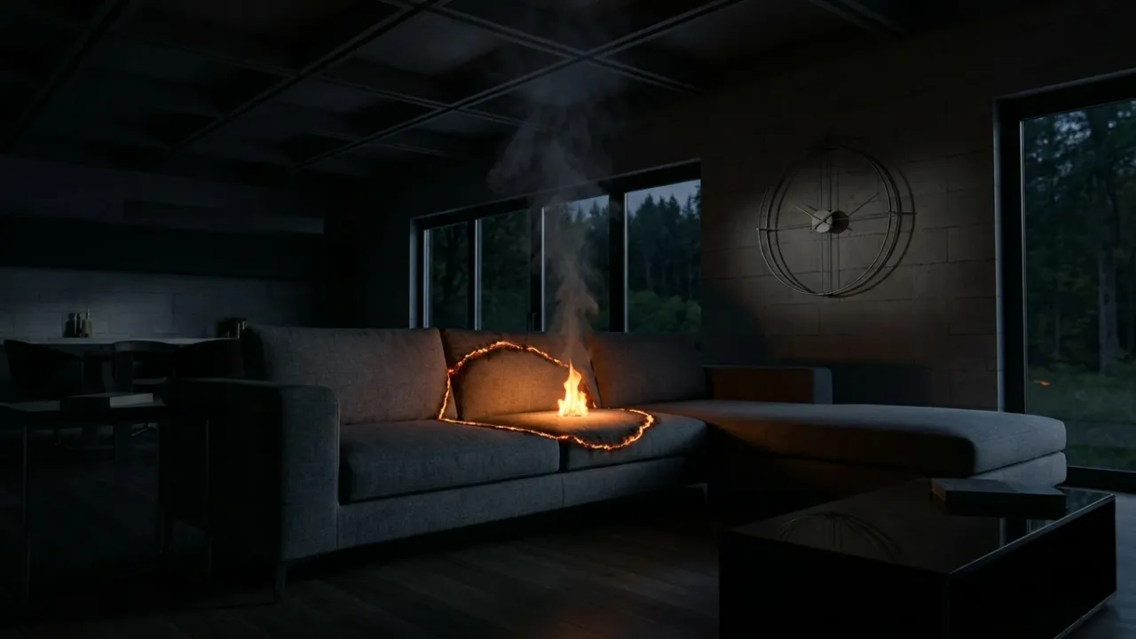
Every escape plan, sprinkler layout, and smoke-control calculation rests on a guess about fire growth. So engineers compress that guess into one short equation. Heat release rate climbs with the square of time, and a single coefficient sets the pace. Pick “slow”, and the design fire needs 600 seconds to reach 1,055 kW. Pick “ultrafast”, and it needs only 75. That one choice often decides whether a building design passes or fails. This post follows the t-squared curve from 1970s detector research to the modern fuels that break it.

TL;DR

• One equation, $\dot{Q} = \alpha t^2$, drives most performance-based fire design.
• Four classes set the pace. Slow reaches 1,055 kW in 600 seconds, medium in 300, fast in 150, ultrafast in 75.
• The square comes from geometry, because a flame front spreading outward at constant speed covers area with the square of time.
• NFPA 72, NFPA 92, NFPA 204, and Eurocode EN 1991-1-2 all share the same fire growth coefficients.
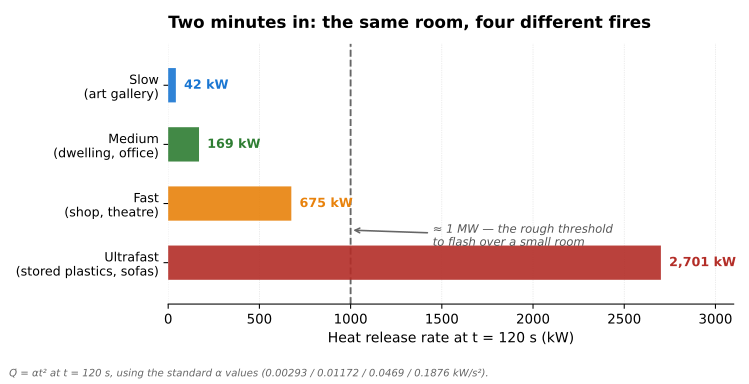
• At 120 seconds the four classes span 42 kW to 2,701 kW — a factor of 64.
• Real incident data give a distribution of fire growth rates, not a constant. Arson alone lifts the 95th percentile by 83%.
• Modern furnished rooms flash over in about 3.5 minutes, against 29.5 minutes for legacy rooms.
• Lithium-ion packs break the model outright. One e-scooter battery hit 1.1 MW in 13 seconds.

What is a t-squared fire?

A t-squared fire names a design fire whose heat release rate grows with the square of time after ignition. Double the clock, and the fire grows fourfold. Everything else follows from one coefficient:

$\dot{Q} = \alpha t^2$

Here $\dot{Q}$ gives heat release rate in kilowatts, $t$ counts seconds after effective ignition, and the fire growth coefficient $\alpha$ carries units of kW/s². So α alone fixes the pace of the whole curve.

Standards then define α through a growth time, $t_g$ — the time a fire needs to reach 1,055 kW. That odd target equals 1,000 Btu per second, a fossil of the model’s American roots. The definition reads:

$\dot{Q} = 1055\left(\frac{t}{t_g}\right)^{2} \qquad \alpha = \frac{1055}{t_g^{\,2}}$

Four named classes then divide the whole design space. Each class halves the growth time of the one above it, so α quadruples at every step.

Class	Growth time $t_g$	α (kW/s²)	Eurocode examples
Slow	600 s	0.00293	Art galleries, public transport spaces
Medium	300 s	0.01172	Dwellings, offices, hotel rooms, classrooms
Fast	150 s	0.0469	Shopping centres, theatres, libraries
Ultrafast	75 s	0.1876	Chemical plants, stored upholstered furniture

That right-hand column comes straight from Annex E of Eurocode EN 1991-1-2. Sources round α a little differently — fast appears as both 0.0469 and 0.04689 — yet the four classes match across NFPA 72, NFPA 92, NFPA 204, and the Eurocode. Few numbers in fire engineering enjoy such broad agreement.

Where did the t-squared fire come from?

The model grew out of fire-detector research in the 1970s. Gunnar Heskestad and Michael Delichatsios ran the key experiments at Factory Mutual Research Corporation for the US National Bureau of Standards, now NIST.

Their 1977 report, Environments of Fire Detectors, landed in two volumes covering measurements and analysis. Together they established the time-squared description of a growing fire. Heskestad also flagged the caveat that still bites today. Real fires pass through an incubation period first, then settle onto the parabola afterwards.

Detection standards adopted the curve first. Beyler carried the analysis into a design method for flaming fire detection, and NFPA 72E picked it up in 1984. Three classes came along: slow, medium, and fast. Ultrafast joined later, then spread into general fire protection work.

From there the curve travelled fast. NFPA 92B took it up for atrium smoke management in 1991, and NFPA 204 applied it to smoke and heat venting. Europe followed through Eurocode EN 1991-1-2. Meanwhile the UK codified equivalent guidance in PD 7974-1, and Australia in its fire engineering guidelines. Fifty years on, a detector-siting tool underwrites structural fire design.

Why does fire growth follow the square of time?

Because circles grow that way. Picture a flame front crossing a carpet at a roughly constant spread velocity $v$. After time $t$, the burning zone covers a circle of radius $r = vt$, so its area comes to:

$A = \pi r^2 = \pi v^2 t^2$

Now give every square metre of that circle the same heat release rate per unit area, $\dot{q}''$. Nothing else varies. Total output then scales with burning area:

$\dot{Q} = \dot{q}''A = \dot{q}''\,\pi v^2 t^2 \propto t^2$

No deep law of combustion appears anywhere in that derivation — only geometry. NFPA’s own commentary puts the same idea in words. A t-squared fire spreads as a circle of steadily growing radius, with constant heat release per unit area across it.

Matching the two expressions also hands engineers a practical dial. Setting $\alpha = \dot{q}''\pi v^2$ and solving for spread rate gives:

$v = \sqrt{\frac{\alpha}{\pi \dot{q}''}}$

That relation lets FDS reproduce a fire growth curve naturally, by spreading flame radially across a surface at the matching speed. No lookup table required.

The derivation fails wherever its two assumptions fail. Rack storage feeds flame upward through stacked plastics, so the burning region grows in three dimensions rather than two. High-rack tests accordingly show growth closer to $t^3$. Discontinuous fuel stalls and then jumps, instead of spreading smoothly. And any surface that accelerates flame, such as a vertical plastic panel, outpaces the square law entirely.

How do engineers handle the slow start?

They shift the time origin. Real fires smoulder, creep, or char for a while before the parabola takes hold, so forcing the curve through the ignition instant misfits the data. The standard fix introduces a virtual origin $t_0$:

$\dot{Q} = \alpha\,(t - t_0)^2$

Fitting then uses only the established growth phase. Before $t_0$ the model says nothing at all, which honestly reflects what test data show.

The same equation integrates cleanly, which matters for fuel bookkeeping. Total energy released during pure growth comes to:

$E = \int_0^t \alpha\,t'^2\,dt' = \frac{\alpha t^3}{3}$

Try it on a medium fire at 300 seconds. The integral gives 0.01172 × 300³ ÷ 3, or roughly 105 MJ. Around 4 kg of plastic, at some 25 MJ/kg, would supply that energy. So a medium curve running past five minutes already demands a serious fuel package — never a wastepaper basket.

Which fire growth class fits which building?

Standards map occupancies straight onto growth classes. Annex E of the Eurocode assigns dwellings, hospital rooms, hotel rooms, offices, and classrooms to medium. Shopping centres, libraries, theatres, and cinemas move up to fast. Chemical plants, alcohol stores, and warehouses of upholstered furniture sit at ultrafast. Art galleries and public transport spaces drop to slow, since sparse fuel sits in a large volume.

Warehouse commodities tell a parallel story in NFPA’s tables. Densely packed paper in cartons earns a slow rating. Mail bags stacked 1.5 m high count as medium, while wood pallets and cartoned plastics burn fast. Plastics stacked above 4 m, and pools of flammable liquid, land firmly in ultrafast.

Furniture data anchor much of this mapping. The European CBUF programme burned more than 1,500 furniture items and materials in the early 1990s, pairing full-scale furniture calorimeter tests with bench-scale cone calorimeter runs. NIST tests on office workstations then showed a pattern worth remembering. Fires open in the slow-to-medium range, then accelerate into fast or ultrafast once flame leaves the first item.

One caution belongs beside every occupancy table. Full-scale free-burn tests at Factory Mutual, plotted against the standard curves, showed that many ordinary fuel arrays beat the medium curve outright. A dry Christmas tree makes the same point at household scale, reaching flashover in about a minute.

What happens after the growth phase?

Nothing in physics lets $\alpha t^2$ run forever, so every design fire needs a ceiling and an ending. The Eurocode builds all three stages into one curve: a t-squared growth phase, a plateau, then a linear decay once 70% of the fire load has burnt away.

Two ceilings compete, and the lower one wins. Fuel supply sets the first. A fuel-controlled fire caps out at the burning area times its heat release per unit area:

$\dot{Q}_{\max} = \dot{q}''\,A_{fire}$

A ventilation-controlled fire caps out on air supply instead. Then the openings rule the fire, not the fuel. US practice uses the classic opening correlation:

$\dot{Q}_{\max} \approx 1500\,A_o\sqrt{H_o}$

Here $A_o$ gives opening area in square metres and $H_o$ opening height in metres. A single doorway 1 m wide and 2 m tall therefore supports roughly 4.2 MW. Most residential rooms consequently turn ventilation-limited soon after flashover.

Skipping this step produces one of the commonest errors in performance-based design. An unbounded ultrafast curve reaches about 17 MW in five minutes and 68 MW in ten, which no ordinary room can supply or sustain. So always cap the parabola, then decide how it decays.

The plateau also changes what the fire growth phase means for the model. Before the cap, α governs everything: detection, tenability, and the smoke layer. After the cap, ventilation and fire load take over, and α barely matters. Escape calculations therefore live almost entirely inside the growth phase, while structural calculations live mostly beyond it.

What does the curve feed downstream?

Four calculation families, all of them load-bearing in modern fire safety design: escape time, detection, smoke control, and structural exposure. Each family takes the same fire growth curve as its opening input, so an argument about α quietly becomes an argument about exit widths, sprinkler spacing, fan capacity, and steel protection at once.

Escape time

Zone models such as CFAST and field models such as FDS burn the design fire, then track when conditions turn untenable. Typical criteria hold visibility above 10 m, gas temperature under roughly 60 °C, and carbon monoxide below about 1,400 ppm, with a fractional effective dose check layered on top.

The available safe escape time must then beat the required safe escape time, with margin to spare. Cooper formalised that comparison in 1982 using a two-zone model built on the same Heskestad and Delichatsios detector work. So the fire growth coefficient propagates directly into exit widths and travel distances.

Detectors and sprinklers

Alpert’s ceiling-jet correlations convert heat release rate, ceiling height, and radial distance into gas temperature and velocity at the device. Evans and Stroup at NBS wrapped them into DETACT-QS. The t-squared variant DETACT-T2 and the vented-compartment model LAVENT both appear in NFPA 204.

Thermal lag then enters through the response time index, or RTI. One caveat deserves attention here. Alpert fitted his correlations largely to fires of 3.8 to 98 MW under high ceilings, so small early-stage fires sit outside that calibration range. Recent modelling nevertheless suggests the design answer stays conservative.

Smoke control

NFPA 92 sizes atrium exhaust from the plume the design fire drives upward. A Heskestad axisymmetric plume correlation, complete with its virtual origin, converts heat release rate into the mass flow entrained up to the smoke-layer interface. That flow then sets the extract rate.

Unsteady t-squared fires approximate real smoke filling better than steady fires do. Still, NFPA 92 works as a starting point rather than a universal answer. Standard axisymmetric correlations can badly under-predict requirements in complex atria, where balconies, spill plumes, and irregular geometry break the assumptions.

Structural fire design

Structural work needs the whole curve, not just its opening. Eurocode Annex E supplies exactly that sequence of growth, plateau, and decay, while PD 7974-1 gives the UK equivalent. The resulting gas temperature history then drives heat transfer into steel or concrete. So one growth coefficient reaches all the way to a column’s fire resistance rating.

How much does the fire growth class matter?

Enormously. At 120 seconds the four curves span a factor of 64 in heat release rate, since α itself covers that same range.

Class	HRR at 120 s	Time to 1 MW	Time to 2 MW
Slow	42 kW	584 s	826 s
Medium	169 kW	292 s	413 s
Fast	675 kW	146 s	207 s
Ultrafast	2,701 kW	73 s	103 s

Read that first column as physical objects. A slow fire at two minutes releases about as much heat as a wastepaper basket. The medium curve matches an armchair getting going. Fast reaches a fully involved sofa. Ultrafast, at 2,701 kW, already threatens flashover in a small room.

Inverting the equation explains the shape of the later columns. Solve for time instead of size:

$t = \sqrt{\frac{\dot{Q}}{\alpha}}$

Time scales with the square root of fire size, so doubling the target size stretches the clock by only 41%. A medium fire takes 292 seconds to reach 1 MW, yet just 413 seconds to reach 2 MW. Each extra megawatt therefore costs less time than the one before it.

Detection shifts just as hard. Ceiling-jet temperature rise scales roughly with $\dot{Q}^{2/3}$, so the same sprinkler sees an ultrafast fire far sooner. Because growth times differ eightfold between slow and ultrafast, activation times separate by minutes. For escape analysis the fire growth class therefore outranks almost every other model input.

Compare that leverage with the inputs engineers usually argue over. Ceiling height, detector spacing, and door width each move the answer by tens of percent. One step in fire growth class moves it by 300%. So the effort belongs in justifying α, not in polishing the third decimal place of a travel-time calculation.

Where does the t-squared fire fail?

Wherever flame spread stops behaving like a growing circle. Four cases matter most in practice, and modern buildings serve up all four.

Modern rooms outrun the old defaults

UL’s Fire Safety Research Institute burned matched living rooms side by side. Each measured about 3.7 m square under a 2.4 m ceiling, and each started with a candle against a polyurethane-foam sectional sofa. The modern room reached flashover in 3 minutes 30 seconds. The legacy room, furnished in natural materials, held out for 29 minutes 30 seconds.

Across three sets of experiments, legacy rooms took at least 700% longer to flash over. Synthetic foam and plastic drive that gap through higher heat release, faster flame spread, and far more fuel per item. So the comfortable “medium” default for a living room now sits on the wrong side of the evidence.

Battery fires skip the growth phase

Thermal runaway feeds itself. Heat accelerates the reaction, the reaction makes more heat, and the cascade needs no help from the room to keep climbing. According to tests by FSRI, UL Solutions, and FDNY, an e-scooter pack of 60 V and 20 Ah, holding 136 cells of 18650 format at full charge, peaked near 1.1 MW just 13 seconds into the event. An upholstered chair in the same rig needs 2 to 3 minutes to reach its peak.

No t-squared curve bends that sharply. Even ultrafast needs 75 seconds to pass 1 MW, roughly six times longer than the pack took. Scale complicates the picture further, since a single 21700 cell at full charge peaks near 3 kW. So a pack behaves nothing like its cells burning politely one after another. For battery storage rooms and micromobility charging areas, measured heat release data must replace the parabola outright.

Real fires refuse to share one α

Studies that fit growth coefficients to real incidents recover distributions, never constants. Holborn, Nolan and Golt analysed the London Fire Brigade real-fire library and fitted lognormal curves with mean fire growth rates from 0.006 to 0.052 kW/s², depending on occupancy. They also reported that α = 0.047 kW/s² covers 95% of fires in public buildings and 89% in retail.

English dwelling fires behave similarly. Hopkin and colleagues derived lognormal fits with means from 0.0022 to 0.0034 kW/s², yet standard deviations from 0.0071 to 0.0132 kW/s². Read those two ranges twice, because the spread runs several times the mean. Baker and co-workers, running Monte Carlo simulations on residential data, approximated α as a triangular distribution from 0 to 0.4120 kW/s², with a mode of 0.0326.

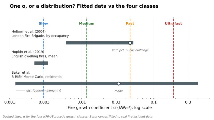
Arson stretches the upper tail further. Nilsson, Johansson and van Hees found that including deliberate ignition raises the 95th-percentile fire growth rate by 83%, and the 99.5th percentile by 110%. A single deterministic curve hides every one of those tails.

Large floors burn by travelling

Open-plan floor plates break the uniform-burning premise. Fires there consume a limited area at any moment and travel across the floor, exposing different structure at different times. Stern-Gottfried and Rein built the Travelling Fires Methodology at Edinburgh for precisely that reason, since uniform design fires — t-squared ones included — misrepresent thermal exposure in big compartments.

How should engineers use the curve today?

Treat the t-squared fire as a sharp tool with a narrow blade. Five habits keep it honest.

1. Question the medium default. Synthetic furniture, plastics, and stacked storage usually justify fast or ultrafast. Demand test data before choosing anything slower.
2. Keep the parabola away from battery fires. Use measured heat release profiles for cells, modules, and packs. Then reserve t² for whatever the battery ignites next.
3. Run a sensitivity study across adjacent fire growth classes. If one step up turns a pass into a fail, the design leans too hard on a single guess. High-consequence buildings deserve a full distribution of α instead.
4. Cap and close the curve. Couple growth to a defensible fuel- or ventilation-limited plateau, then a decay phase. Unbounded t² growth means nothing physically.
5. Check travelling fires on large open plans. For big floor plates, a uniform t² fire can understate the exposure that governs structural design.

The t-squared fire earns its long life: two parameters, one honest idea about spreading flame, and five decades of service in standards on three continents. Yet fuels changed faster than the standards did. Foam sofas, stacked plastics, and battery packs all outrun the classes drawn in 1977. So use the curve where the geometry holds, and know in advance where fire growth breaks the parabola.

Cite this article

Dinh, D. C. (2026, July 21). The t-Squared Fire: How Fire Growth Rate Shapes Escape Time (Updated July 25, 2026). PyroRisk. https://pyrorisk.net/blog/t-squared-fire-growth-slow-medium-fast-ultrafast/

Get citation →

---